Groundwater Potential Mapping

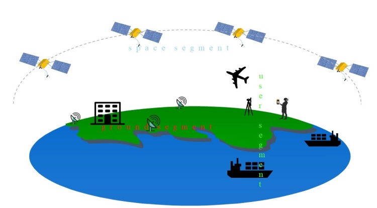
Mapping of groundwater is essential in planning of water resources development, use, and management. The knowhow of potential distribution of available groundwater bodies is hence vital here. The mapping of amount of permanent water resources in aquifers can produce the groundwater potential distribution. Remote sensing and geographic information system (GIS) in combination with vertical electrical sounding (VES) can be applied for groundwater zoning and validation.

1. Derivation of contributing factors

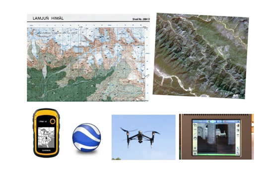
For groundwater prospect zoning, parameters such as; geology (GE), geomorphology (GM), land use land cover (LULC), lineament (LI), slope (SL), drainage (DD), and normalized difference vegetation index (NDVI) has to be considered. These parameters can be derived from satellite images, ancillary data, and field studies. GE maps can be collected from government agency, while GM, DD and SL can be derived from digital elevation model (DEM). However, the print of geology map has to be geo-referenced and digitized. Further, LULC and NDVI can be generated from satellites images using multi-spectral bands of optical remote sensing.

Geology and Geomorphology

Geology of the area provides hint in groundwater distribution. The groundwater distribution depends on the type of subsurface lithology and underlying geological structure. If the area has major geological structure such as fracture, faults, and outcrops etc., which intrudes the groundwater flow and helps in storing the water percolated from surface.Similarly, geomorphological features of any region determine the types of landform and the process that control the movement of groundwater.

Drainage and Lineament Density (km/km²)

Drainage Density is defined as the ratio of total length of all the streams within the basin to the total area of basin. Higher the drainage density, lesser the infiltration and more prominent to runoff and vise-versa. Similarly, lineament is outcome of visual interpretation of satellite images where curvilinear and linear appearances can be delineation. It shows anomalies of subsurface lithographical structure, outcrops, ridges etc. Higher the lineament density provides greater storage capability through secondary porosity.

LULC and NDVI

LULC is an essential indicator for the management of natural resources and groundwater extent. NDVI is calculated using Near Infrared (NIR) and red (R) bands of multi-spectral images of optical remote sensing. NDVI = (NIR-R)/(NIR+R). The values of NDVI range from -1 to +1 in which -1 to 0 indicate barren land with infrastructural developmental activities in the region. Water bodies lies in mid values around zero. Values from +0.5 to +0.8 represent the green land which indicate the presence of groundwater.

Slope and Topography

The slope gives the hydro-geological characteristic of the groundwater. Higher the slope angles, more prominent to surface runoff and less time for the surface water and precipitation to infiltrate through subsurface. Topography with more ruggedness and gentle slopes can have different water storage capacities. Here, an earthquake can change the topography and hence the distribution of ground water.

Flow chart for overall method for ground water potential mapping (S. GYELTSHEN ET AL. 2019)

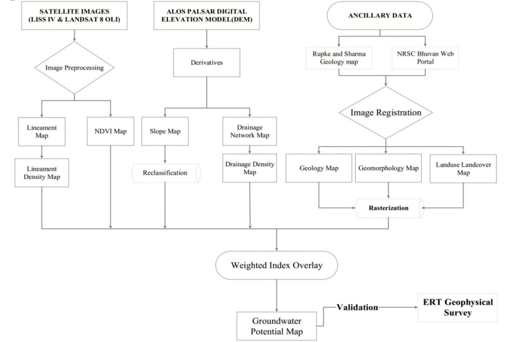
2. Ground Water Potential Index (GWPI)

The weighted overlay technique, which is frequently used in GIS, and can be applied to determine the GWPI. The method is the straightforward combination different type of thematic layers (parameters as defined above). This algorithm considers the importance and effectiveness of individual thematic layers for the generation of potential map.

There are numerous weighting techniques like analytical hierarchical process (AHP), regression models, and indexing methods to determine individual weights of sub-class to reduce human bias. Similarly, ratings are provided to sub-classes of each factors based on their potential of having ground water. Sub-classes having higher potential get more rating and vice-versa.

GWPI is summation of product of weight and rating of each thematic layers. The weighted index overlay technique to determine GWPI can be expressed mathematically as:

where, ‘W’ represents the weight of individual layer (i),
‘R’ the rating of individual layer (i),
‘n’ represents total number of thematic layers.

3. Validation of GWPI map

The GWPI map produced can be compared with water column map generated tube-wells. Other ground data assembled during drilling, and geophysical survey can also be considered for validation of result. Again, the water level fluctuates for monsoon and other periods so field data collection from tube wells should consider seasonality. VES studies the resistivity or conductivity of sub-surface materials whose data can also be applied for the purpose of validation.

– Sangay Gyeltshen

Author is researcher from Bhutan and this work was carried out during his Post Graduate studies in RS and GIS (2018-2019). He can be found at sangye89@gmail.com.

Downloading 12.5m DEM (ALOS PALSAR)

Alaska Satellite Facility

Alaska Satellite Facility (ASF) is very good resource center for providing remote sensing datasets specially SAR data and related products. It have data archives of past 25 years. ALOS PALSAR radiometric terrain corrected (RTC) high resolution (HR) product is one among the SAR data products of ASF. It’s one major component is Digital Elevation Model (DEM) which have spatial resolution of 12.5m. More information about ASF datasets can be obtained from its website.

When you click the ALOS PALSAR-RTC product you will be directed to a new page that will give description about its various products. You can see its global coverage map as well.

Click the find data option available to download the datasets. You will be redirected to the ASF data search vertex. You can also reach to this page by searching ASF Data Search in Google. There you can explore the options of different datasets available to download.

Stages to download data

‘Sign in’ with your user name and password. If you don’t have it you can register for one very easily to get your username and password.
In ‘search type’ select geographic. In ‘dataset’, select ALOS PALSAR. Then navigate to your area of interest and zoom it.
There are different options for drawing shape in ‘selection shape’ button either as point, line, polygon, or rectangle.
Select any of these options and draw point or polygon on your research area. (Yellow polygon in picture below)
Then click ‘search’ button.
Here you will get the list of ‘scenes’ for your area of interest. Along, with scenes there are ‘scene detail’ and ‘files’ included in the particular scene selected.
You can click on any scenes to know where it is located in map (red highlighted scene in picture). Then form the list of ‘files’ click the download button beside the ‘Hi-Res Terrain corrected’ option to download the file
Once the product is downloaded. You can unzip the folder and open the product in GIS software. The DEM you require is with extension of ‘.dem.tif’.
Check the DEM you have downloaded. If it contains numerous voids, particularly in your area of interest, you can download DEM from another year.

Global Navigation Satellite System

The position at a point on earth surface is given by its latitude and longitude measured from a certain datum. This position along with time information is of great use in mobility of ships in the ocean, transportation of vehicles, agriculture, navigation, and mobile communications. There are many other applications that require positioning information. There are certain constellations of satellites designated to provide such location and time information at any time of day or night and at any location of earth. Such a system of satellites are known as global satellite navigation systems (GNSS). GNSS is a network of satellites that continuously transmit coded information, which makes it possible to precisely identify locations on earth by measuring distance from the satellites. A system of 18-30 satellites orbiting in medium earth orbit can be able to provide the global coverage of location information. The global positioning system (GPS) which is widely used for positioning and navigation is one of GNSS. Besides, there are other global and regional satellite positioning and navigating systems. Originally such positioning and navigating systems were developed for security purposes but later on the services were also provided to civilians. The difference would be in terms of accuracy where the civilians would receive lesser accuracy services from GNSS.

Segments in GNSS

The structure of any GNSS is composed on mainly three segments that are

Space segment:
Space segment can be taken as satellite segment. This consists a constellation of satellites, specially built for positioning services, orbiting in space. The availability total satellites of deemed constellation size can provide continuous signals for precise positioning. They are located in their respective orbits generally medium earth orbits and/or geostationary orbits. The spacing between satellites and the orientation of satellites are maintained so as to receive accurate signals. When higher number of satellites are visible from ground receiver the accuracy gets higher. Respective agencies of GNSS regulate the operation of satellites. It includes regulation, maintenance, and replacement the satellites.
Control Segment:
Control segment includes the infrastructures on the ground in to monitor the satellite and control the data transmission. This segment consists of major control station, ground antennas and some monitoring station. The satellite paths are tracked by monitoring stations and communicate the conditions to the major control station. Then the control station works to maintain the accuracy of satellite signals via the ground antennas. The ground control segment maintains the health of the satellite to so that they can transmit accurate signals. So, the control segment track the satellites, update their orbiting positions, and calibrate and synchronizes the clocks in satellites.
User Segment:
User segment consists of any entity that used the navigation and positioning services of GNSS. GNSS were at first developed for military purposes so the military are foremost users that benefits the precise positioning provided by the satellites. The broad users includes civilians, public or private firms, and scientific community using GNSS for research, tracking, navigation, surveillance and so on. The difference in military and civilian use of satellite positioning would be in accuracy where former gets benefits of cm level accuracy. The GNSS receiver are nowadays integrated in smartphones, watches, and vehicles having numbers of applications. The accuracy may depend upon the surrounding of the users and the type of receiver used. So, the user segment consists of receiver equipment, applications, and computation of the positioning data.

Applications of GNSS

There are numerous applications of GNSS as it gives positioning and time information.

To find precise location information (latitude, longitude, elevation, and time)
Scientific researches for time and travel measurements
Military services for defence activities
Survey with tools like Differential GPS (DGPS) and Real time kinematic DGPS (RTK DGPS)
Marine navigation and air transport navigation as well as tracking vehicle tracking
Speed measurements with tracking of vehicles on roads
Search and rescue operations
Recreation purposes

GNSS around the Globe

Global positioning system (GPS)

GPS belongs to United States which was originally called NAVSTAR GPS. First GPS satellite was launched in 1978 by US Department of Defense for military use. By mid 1990s it reached a constellation of 24 satellites to have global coverage. GPS provides navigation and timing information. The services was provided to civilians in 1980s with intentionally degraded quality of signals. By 2000 there were more civilian users than military users, and this trend was increasing as years passes by. Since there was increase in numbers of civilian use of GPS, higher accuracy GPS service was also provided to civilians. GPS provides accuracy of greater than 3.5 m.

GLObal NAvigation Satellite System (GLONASS)

GLONASS belongs to Russian which was started during former Soviet. The development of GLONASS began in 1976 and the satellites were launched in the year 1982. In mid 1990s GLONASS reached its full potential. Due to less life time those satellites have to be replaced. Now third generation of GLONASS satellites have deployed that have lifespan of 10 years are more accurate and weighs less than its predecessors. GLONASS now have 24 operational satellites in its constellation and have global coverage. The service from GLONASS was accessible to civilians from 2007. Civilians get standard positioning service from GLONASS whereas Precise Positioning Service (higher accuracy) is limited to military and authorized users. The accuracy of GLONASS can be up to 2.8 m.

BeiDou Navigation Satellite Systems (BDS)

BDS belongs to China. First generation of BeiDou-1 satellites were launched in 2000 as experimental satellites to provide navigation service. By December 2012 second generation satellites of BeiDou-2 reached 16-satellite constellation to cover regions of the Asia and Pacific. Third generation of Beidou-3 satellites were deployed for global coverage in 2015. It started to provide global service in December 2018. Recently in on June 23 2020 a satellite was launched to complete its constellation of third generation BeiDou-3 satellites. So, there are now 30 Beidou-3 satellites in it constellation. The services provided by BDS are for public use (open) and military purpose (restricted). The civilian service has accuracy of 10 m location tracking accuracy whereas the restricted military service has location accuracy of 10 cm.

Galileo Satellite Navigation

Galileo positioning system is a GNSS of European Union with its primary users as civilians rather than military. First satellite of Galileo GNSS constellation was launched in 2011. The constellation size of Galileo is of 30 satellites. It started to provide its service by 2016. In 2018 it reached number of 26 operational satellites to provide global coverage. Its accuracy is of 1m available to public whereas the encrypted signals have accuracy of (1 cm).

Navigation with Indian Constellation (NAVIC)

NavIC is regional navigation system that belongs to India. The launch first satellite of IRNSS was on 2018. There are 7 satellites in its constellation. NavIC covers area of India and region extending 1500 km around it, which is its primary service area. An Extended Service Area lies between primary service area and area enclosed by the rectangle from Latitude 30^oS to 50^oN, Longitude 30^oE to 130^oE. ISRO plans to increase the constellation size from 7 to 11 and also the ground coverage. NaVIC also provides two levels of services, one to civilians and other for military or authorized use. The IRNSS System is expected to provide a position accuracy of better than 10 m in India and 20 m in the primary service area.

Quasi-Zenith Satellite System (QZSS)

QZSS is another regional satellite navigation system belonging to Japan. It covers the area of Japan and the Asia-Oceania region. Its first satellite was launched in 2010. QZSS started to provide its service in 2018 with four satellites. There are plans to increase its number to 7 by 2023.

Coordinate Systems Used in Nepal

In Nepal most of the spatial data and maps are based on two Global Coordinate System (GCS) as a reference. The first one is Everest 1830 which is mostly used in topographic maps and maps produced by governmental agencies like Department of Survey. The second one is WGS84 as most of the images and maps available over the internet are referenced in this system.

GCS	Everest_1830	WGS_1984
Angular Unit	Degree (0.0174532925199433)	Degree (0.0174532925199433)
Prime Meridian	Greenwich (0.0)	Greenwich (0.0)
Datum	D_Everest_1830	D_WGS_1984
Spheroid	Everest_1830	WGS_1984
Semi-major Axis	6377299.36	6378137
Semi-minor Axis	6356098.352	6356752.314
Inverse Flattening	300.8017	298.2572236

In Projected Coordinate System (PCS) of Nepal the projection system used is universal transverse Mercator (UTM) which may be based on either WGS84 or Everest 1830. Considering the WGS84 Nepal lies in two zones of UTM projection system which are 44 north and 45 north zones. The former zone covers western half of Nepal whereas latter zone covers the eastern half of the country. Similarly, when UTM is based on Everest 1830 the two zones are modified into three zones differentiated by longitude of the coordinate as 81, 84, and 87. Each of these three zones of modified UTM (MUTM) covers west, central and eastern Nepal respectively. When one creates customized PCS one must make sure of GCS being selected as mentioned in previous lines. Following are the details PCS used in Nepal.

WGS 1984 based PCS

Zones	UTM_44N	UTM_45N
Projection	Transverse Mercator	Transverse Mercator
False Easting	500000	500000
False Northing	0	0
Central Meridian	81	87
Scale Factor	0.9996	0.9996
Latitude of Origin	0	0
Linear Unit	1	1
GCS	WGS 1984	WGS 1984

Everest 1830 based PCS

Zones	MUTM_81	MUTM_84	MUTM_87
Projection	Transverse Mercator	Transverse Mercator	Transverse Mercator
False Easting	500000	500000	500000
False Northing	0	0	0
Central Meridian	81	84	87
Scale Factor	0.9999	0.9999	0.9999
Latitude of Origin	0	0	0
Linear Unit	1	1	1
GCS	Everest 1830	Everest 1830	Everest 1830

Coordinate Transformations

There is slight difference between these two types of PCS used in Nepal. If you use two different PCS based files/datasets in same analysis you can observe that the boundaries of same features are not exactly overlaying. To avoid this you need to make sure the PCS for all features or layers under analysis are in same PCS. If the coordinate system are different you can do geographic transformation from one PCS to the required one. Once all the datasets are in same PCS then only you can start data analysis with no errors due to coordinate systems.

In Nepal the PCS are based on two datum i.e., WGS84 and Everest 1830. So, here we do datum transformation from one GCS to another. If you want your data layers to be in WGS84 UTM_44N or 45N, there is need to transformation from Everest 1830 to WGS 1984. We use following method and parameters.

Source GCS: Everest 1830 and Target GCS: WGS 1984
Method: Molodensky
Translation parameters:
Translation along X axis (in meters) = 293.17
Translation along Y axis (in meters) = 726.18
Translation along Z axis (in meters) = 245.36

In order to do geographic transformation from WGS 1984 (Source GCS) to Everest 1830 (Target GCS) we use same method with same values with negative signs in front.

Digital Elevation Model

Height on a certain point of the earth surface is represented by an elevation above certain datum such as mean sea level. This elevation varies as one tend to move from one point to another on surface of earth. The earth surface is highly undulate which cause these variations in the heights. Elevation of earth surface thus becomes continuously varying. This height information can be represented digitally in vector formats or raster formats.

Representation of elevation

Vector formats:
The vector formats of height representation can be observed in topographic maps in form of points or lines. The point in such maps are referred to as spot heights which provides height information of certain location either building or a hill top. The lines in topographic maps that reveal height information are known as contours. Contours are the lines formed from connections of points having same height. Besides one of important vector format for terrain representation is triangulated irregular network (TIN).
Triangulated Irregular Network:
TIN is formed from a set of triangles that are non-overlapping whose vertices carry the elevation information. TIN can be formed by the process of triangulation where most commonly used one is Delaunay triangulation. A Delaunay triangulation is a set of linked but non-overlapping triangles. One condition in this triangulation is that the circumscribing circle of each triangle should not include any other points. During formation TIN each of the triangles tend to become as nearly equilateral as possible. The interpolation of TIN produces DEM which is grid based surface model.
Raster formats:
The raster formats of height representation can be obtained from satellite imageries. This can also be formed by interpolation of contours and spot heights. The raster format is a continuous surface formed by grids or cells. Each cell value has the height information of that particular location. So a single elevation represents the entire area of the cell and this necessitates the requirement of finer spatial resolution of cell for greater accuracy. Digital Elevation Model (DEM) that we use is in this format.

DEM

A digital elevation model (DEM) is a 3 dimensional representation of a terrain’ surface created from a terrain’s elevation data. The elevation can be measured from any reference datum. Topography of the earth’s surface is expressed in form of DEM. Hence the DEM can give basic information of topography such as elevation, slope and aspect of a terrain. Besides, features like drainage basins and stream network can also be produced from DEM. DEMs are widely used in hydrologic and geologic analyses, hazard monitoring, natural resources exploration, agricultural management etc.

DEM is often used as a generic term for elevation models only representing height information without any further definition about the surface. Thus, DEM can be further differentiated into digital surface model (DSM) and digital terrain model (DTM).

DSM

DSM stands for digital surface model. It counts height of the surface of the bare earth as well as the features lying above it like trees, buildings, and other structures. DSM used for landscape modeling, city modeling and visualization applications.

DTM

DTM stands for digital terrain model. It is bare earth model. DTM represents earth’s surface without vegetation, buildings, etc. DTM is used for flood modeling, watershed modeling, geological applications, and so on. DBTM (or Digital Basement Terrain Model) is the digital representation of the basement surface.

Techniques to generate DEM

Following is the list of techniques used to create DEM.

DEM can be produced from already existing data like topographic maps that contains height information in the form of contours, or spot height. Geo-referencing such maps and digitization of contours and spot height convert existing data into digital format which can be converted into DEM by interpolation methods.
Field measurements of heights with the help of total station theodolites and GPS gives you direct measurement of height of height information for existing terrains which can be imported into GIS software and converted into DEM.
Aerial and satellite images are another sources for DEM. Photogrammetry use stereo pair of images that are taken either from atmosphere or space to produce DEM. Stereo pairs of SPOT satellites had been used to produce DEM since its launch. ASTER DEM was also produced form stereo pairs of Advanced Spaceborne Thermal Emission and Reflection Radiometer (ASTER) instrument of the Terra Satellite. ALOS World 3D is produced from Panchromatic Remote-sensing Instrument for Stereo Mapping (PRISM), which was an optical sensor on board the Advanced Land Observing Satellite “ALOS”
Light detection and ranging (LiDAR) is another promising technique for generation of DEM. Differences in laser return times and wavelengths in LiDAR is used to make digital 3D representations of the target. Sometimes called as 3D laser scanners, LiDAR are used to produce very high resolution DEM used for a particular location or structures.
Radar (stands for radio detection and ranging) locate the position by transmitting, recording, and processing the radio signals. The generation of DEM is one of numerous applications of radar.
Interferometric Synthetic Aperture Radar (InSAR) produces DEM by use of double pass of radar satellite for a particular location. Most of the DEM data available today are products of InSAR microwave remote sensing. Shuttle Radar Topography Mission (SRTM) was equipped with two antennas to generate interferometric data. SRTM DEM is widely used worldwide.
The laser altimeters are also used to model the surfaces of moon and mars. Mars Orbiter Laser Altimeter (MOLA) is one of instrument in Mars Global Surveyor (MGS) that had been used to create DTM for mars. Similarly, Lunar Orbiter Laser Altimeter (LOLA) is an instrument embedded in Lunar Reconnaissance Orbiter (LRO) had been used to produce the DTM for lunar surfaces.

Links to download DEM

Here are some links to access freely available DEM sources. You may need to register to download these data-sets.

SRTM DEM (30 m of USGS can be downloaded from Earth Explorer),
ASTER DEM (30 m can be downloaded from Earth Explorer),
ALOS World 3D (30 m DEM provided by JAXA, Japan),
MOLA DEM (surface terrain model for Mars),
Open Topography (LiDAR data, many other resources and softwares),
ALOS PALSAR RTC (A 12.5 m DEM provided by Alaska Satellite Facility)
TanDEM-X (a 90 m DEM provided by DLR, Germany)

Coordinate Systems

Coordinate of an entity is the most important feature of data in GIS and remote sensing. This only can make possible the exact location of each feature expressed by the data. In a simple Cartesian coordinate system there are x axis and y axis intersecting at right angle where the intersecting point is origin. The location of a point in Cartesian surface is determined by its relative position from origin in x axis and y axis. In similar way, on surface of the earth the equatorial plane and central meridian plane forms x axis and y axis respectively. The location here is given in terms of longitude and latitude, which are an angular measurements made by the intersecting planes.

Longitude and Latitude

Longitude is the angle is made by intersection between a central meridian plane and any other meridian plane whereas latitude is the angle made by the intersection between equatorial plane and an imaginary line coming from the point of interest. The intersection at both case should pass from the central point of the earth. This can be further clarified from following figure.

Here in above figure O is the center of the earth and WPEQ is the equatorial plane, whereas NPSQ is the central meridian plane, and N, S, W, and E are four directions. Now as we move east from point P the angle will increase and reach 90^o at E and 180^o at Q and it also same if we move west. These angle at a particular location gives a measure of longitude. Longitude ranges from +180 (or 180° E) to -180° (or 180° W). Similarly, if we move north from point P the angle will increase and reach 90^o at N and is same while one moves south. These angles at particular location moving north or south from equator gives a measure of latitude. Latitude ranges from +90° (or 90° N) at the North Pole to -90° (or 90° S) at the South Pole.

General types of coordinate systems

Longitude and latitude makes the coordinates of earth surface and co-ordinate of a point depends on its datum and projection. A datum is frame of reference for measuring locations on the surface of earth. So far different ellipsoids have been developed closely fitting to the surface of earth either or a part of it and they are called datum. When datum is closely fitting to the entire surface of earth, they are global datum and when they are closely fitting to a particular portion of the surface of earth they are called local datum. Projection is the method of converting the coordinate system from the spherical surface of the earth to the planar surface. In projection a three dimensional surface information is transformed into a two dimensional information. Co-ordinate of the same point differs when either its datum is changed or its projection is changed or parameters of projection are changed. Thus, based on various datum and projections methods there are numbers of coordinate systems.

The following are two common types of coordinate systems used in GIS:

Global coordinate system (GCS): In GCS an earth is considered as a spheroid or ellipsoid, where longitude and latitude are a measuring unit of the coordinate system. Some of such coordinate system are developed to fit the particular part of the earth surface, so it can provide faulty readings on area which it is not fitting properly. As an example Everest 1830 is a GCS that have good fit for countries in South and Southeast Asia, Airy 1830 is used in Great Britain, NAD83 epoch 2010.00 for North America. These ellipsoid not necessarily perfectly fits the whole earth. There are many such local GCS that may not fits properly to neighboring nations. To avoid this there is development of CGS that fits the whole globe and this was achieved with numerous satellite observations and datasets from global Navigation Satellite System (GLNASS). International Terrestrial Reference Frame (ITRF), Geodetic Reference System 1980 (GRS80) and World Geodetic System 1984 (WGS84) are some such examples that have global coverage. The WGS84 GCS is the most commonly used references.

Projected coordinate System (PCS): Projection simply means estimation of something from an existing data. In case of coordinate system projection refers to translation of surface coordinates of earth into a map or screen. Thus the coordinate system used in mapping for a particular area is projected coordinate system whose reference is based on GCS. In PCS a position on earth’s surface is measured in the terms of x co-ordinate and y co-ordinate or easting and northing using linear unit of measurement from an assumed origin. Maps are flat, but the surfaces they represent are curved so there are unavoidable distortions in at least one of the properties of a map: either shape, area, distance, or direction. There are numbers of methods for projection. There are different projections methods like conic projection, cylindrical projection, planar projection, and so on. Some examples of PCS are universal transverse Mercator (UTM), Albers Equal Area, or Robinson. UTM is most widely used cylindrical projection method.

Free and Open Source Software (FOSS) for GIS

People doing remote sensing and GIS analysis should be grateful for many freely available software around the world and huge numbers of peoples volunteering to develop them. So using FOSS, will not only save your money but these many people in background will solve your problems.

An open source application by definition is software that you can freely access and modify the source code for. Open source projects typically are worked on by a community of volunteer programmers. Open source GIS programs are based on different base programming languages. A GIS software lets you store, retrieve, analyze, interpret, and produce maps from spatial data.

According to Free Software Foundation (FSF) software can be labelled as free if software if the associated license conditions fulfill the “Free Software Definition”, which grants four freedoms:

The freedom to run the program, for any purpose.
The freedom to study how the program works, and adapt it to your needs.
The freedom to redistribute copies so you can help your neighbor.
The freedom to improve the program, and to release your improvements to the public, so that the whole community benefits.

Following is the lists of some popular FOSS for GIS and remote sensing:

QGIS

QGIS is which was also known as Quantum GIS can be freely downloaded and installed from its website. This software is tough competitor for commercial GIS software. There are numerous options for data processing like spatial analysis, terrain analysis, resource mapping, cartographic applications, and map production to name a few. If you think commercial software are too expensive then QGIS your best alternative. One of the best thing in QGIS is its library of plugins, using which one can do some extraordinary tasks. For example, with SCP plugin one can download Landsat and/or Sentinel-2 images, carry out image pre-processing, and image classification along with post classification accuracy measurement and change analysis. The plugins are developed by QGIS community voluntarily and if you cannot find certain analysis tools you can always search for plugins and install them as per your need. This volunteer participation in development of QGIS is its foundation of success.

SNAP

With advent of freely available imageries of European space agency (ESA) there was also development of sentinel application platform (SNAP). The SNAP software is also freely available. This software has the capabilities to process multispectral as well as microwave remote sensing data. With installation of SNAP you can process whole scene of an image in a step by step manner. So, if you have data of optical satellites, or radar satellites SNAP is the best choice in freely available software. SNAP also possess the plugins necessary to carry image processing smoothly.

GRASS GIS

GRASS stands for Geographic Resources Analysis Support System (GRASS) and this software was at first designed and developed by the US Army Corps of Engineers as a tool for land management and environmental planning. It is the public domain GIS software application, probably the most well-known open source and original GIS software applications. In GRASS software one can process raster-based data, vector-based data, do an image processing, produce graphics images, and conduct spatial modeling. This freely downloadable GIS software can also be used for database management. Users looking for software that specializes in terrain manipulation should consider GRASS as a top option. GRASS GIS can be your primary option for data analysis, image processing, terrain modelling, and statistical analysis of spatial data.

SAGA GIS

SAGA stands for System for Automated Geoscientific Analysis. SAGA is one of the classics in the world of free and open-source GIS which you can just download package and click the graphical user interface (GUI) file to open the visualization and analysis widow. SAGA has an intuitive that lets users manage and visualize geographic data with graphs, histograms and maps. It started out primarily for terrain analysis such as hillshading, watershed extraction and visibility analysis. Now, SAGA GIS is a powerhouse because it delivers a fast growing set of geoscientific methods to the geoscientific community. Terrain modeling with DEM is the strength of SAGA. Besides, numerous functions are added in newer versions for image analysis, interpretation, feature extraction, and LULC classification.

ILWIS

ILWIS, stands for Integrated Land and Water Information System, is one of the oldest software for hydrological and watershed analysis. ILWIS is good at the basics – digitizing, editing, displaying geographic data. Further to this, it’s also used for remote sensing with tools for image classification, enhancements and spectral band manipulation. This was once commercial software and is nicely documented with manuals and user guides. Thus, with such resources one would readily enjoys this free software. It is recommended for watershed managers and planners.

Diva GIS

Diva GIS specializes in mapping biological richness and diversity distribution including DNA data. So, all the scientist doing research in biological sciences this free software might be of your interest. This Diva package have capabilities of mapping and analyzing data. Using Diva GIS one can extract climate data for all locations on the research area. Then you can carry out the statistical analysis, and modeling.

gvSIG

The software gvSIG has easy-to-use interface where users can create layouts and access geoprocessing networks. gvSIG is an outlet for numerous professionals in open-source network of geomatics. 3D visualization and animation is also made possible in gvSIG due to which users can view all layer types in 3D vector and raster layers. It can be considered best option after QGIS as it has features like desktop app, field app, along with capabilities of 3D. So, if you are in field work and requires GIS software installed gvSIG is perfect.

Whitebox GAT

Whitebox GAT (Geospatial Analysis Toolbox) is another free GIS software to carry out advanced geospatial data analysis. One can carry out the operation of GIS like clip, convert, analyze, manage, buffer, extract among hundreds of its functions. The raster operations for terrain analysis and watershed analysis are its strengths. Besides it can also be used in analysis of satellite images where its key component is analysis of Light Detection and Ranging (LIDAR) data. The LiDAR toolbox is a life-saver. The capacity to process LIDAR data increases its accuracy in terrain and hydrodynamic modelling. It has applications in both environmental research and the geomatics industry. Whitebox GAT also provides functionality for storm surge modeling, hydrodynamic modeling, and shoreline mapping.

There are many other softwares which you can explore. MapWindow GIS, openJUMP, orbisGIS, GMT Maping Tools, TNT Lite, GeoDa, FlowMap, uDig, OpenStreetMap, HecRAS, Google Earth, etc are some to name.

Data sources for GIS

Data is one of the key component of GIS. It contains the location along with various other features/attributes. This location information helps to pinpoint its relative position of the data on the earth and be further analyzed with the help of attribute information. These data can be derived from various sources. People can use topographic maps, aerial photographs, satellite imageries, information obtained from ground surveys, readily available reports and government or research publications. Following are some lists.

Webpages:

There are different web portals hosted by NASA, ESA, and other space agencies where one can download free imageries, aerial photographs, and DEMs. Some of such web portals are EarthExplorer, GLOVIS, and Alaska satellite facility.

Map-sheets:

Hard copy maps and their scanned copies; aerial photographs; and digital data files. E.g. sometimes referred to as analogue maps can also be sources of different spatial data. The digitization procedures of such maps can produce vector and raster data.

Global Positioning System (GPS):

GPS is determining accurate positions on the surface of the earth computes positions from signals received from a series of satellites. There are many hand-held devices to track the one’s GPS and the data stored in such devices can be retrieved in form of waypoints, tracks, and polygons. Nowadays, GPS is embedded in smartphones and smart-watches as well which can prove useful in crowdsourcing data.

Remote Sensing:

Remotely-sensed imagery; point data cloud, samples from remote surveys; are rich sources of RS/GIS data. Satellites, UAV and drones, laser scanners, are some tools to produce such database.

Field Survey:

While doing any kind of field surveys geo-tagged data can be easily analyzed in GIS software. Distance is measured using pedometer, chains and tapes. The direction measurements were made with transits and theodolites. The total station captures distance and direction data in digital form. Laser scanners for imaging 3D structures, drones and UAVs.

Other Sources:

Besides there are many ways to build RS/GIS data. Like: GIS data from libraries, data from mapping agencies, elevation data, bathymetry data, georeferenced images, state and national agencies, and detailed district/ municipal data.

Downloading Sentinel-2 Data Products

Go to the website: https://scihub.copernicus.eu/dhus/#/home
Sign up and create your account, verify your account via your email.
Then log in with your username and password.
Navigate to your area of interest and draw your area. Here two buttons will help you.The top button is for navigation and the bottom one is for drawing polygons. They can be toggled by just clicking.
Then there is menu button on top left, by clicking it you will get search-criteria window. It have search button on top right which can be clicked after filling the criteria.
There in advanced search, you can choose the method by which you want to search your data. So, select sort by sensing date and put the start and end date of sensing period. Then, select satellite missions as per your data interest.
If you select sentinel-2 then you can choose satellite platform either 2A or 2B. If you want to view images of both platform leave it blank.
Then select product type as S2MSI1C or of your interest.
Write cloud cover in this style [0 TO 20] where the range can be as per your requirement.
Then click on search button on top left of this criteria window and you will get list of images. You can select image you want to view and click zoom to product button available there.
There is a button with eye by clicking which you can see metadata of the image file. There you will see the foot print of your image a quick-look image and attributes. In attributes you can know the cloud cover percentage of the scene. If your requirements are matched you can download the image from there.
Besides, there is basket button to add the product into your basket. Sometimes, the data are not available online at the moment you are searching so you can add the image produce in your cart and download later whenever available.
Or you can download the image file by clicking the download button. Since the image contains numerous bands its size can be large so it will take some time to get download.

Data Models in GIS

A. GIS data types

GIS can be thought of as a system of hardware and software wherein geographically referenced data (spatial data) and associated attributes (non-spatial data) can be captured for manipulation, analysis, and modelling to assist and speed up decision making and management task (Joseph and Chockalingam, 2018). This definition mention two basic types of data used in GIS. Spatial data describes the absolute and relative location of geographic features. Whereas, attribute data describes characteristics of the spatial features. Here spatial data gives answers of where and attribute data tries to answer of what for a certain feature on the earth surface.

1. Spatial data

First is the spatial data which consists the location information. These can be point of a certain earth features, or a line representing linear features like road or river, polygons that reflects area covered by certain land use type, and surface features representing the elevation of surface. Such spatial data can be discrete or continuous depending upon the type of feature it is representing. Information of buildings and roads can be discrete while meteorological information like temperature, and rainfall represents continuous spatial data. These spatial data can be represented by vector and raster data formats. In the left side of following image there are certain polygons that represent area of villages that are adjacent to a river shown by linear features.

2. Attribute data

Second one is attribute data that explains the characteristics of certain geographical features. These characteristics can be quantitative and/or qualitative in nature. Attribute data is often referred to as tabular data. It is non-spatial data as it only consists of textual information that describes the geographic entity without revealing their information. Characteristics like height of building, length of roads, area of forests, and so on can be compiled as tabular format and expressed as attribute data. In above figure there is a table that represent attribute data as it consists information of id, shape, and name of spatial features. Further data regarding the area of each features, and other characteristics can also be added in this table.

B. Data Models

A model is the simplified representation of the real world phenomena or a system. The representation of a certain location in one’s mind can varies from others’ perspectives so it will create problems while such conceptual models are to be shared. To share models there should be some uniformity and in case of earth representation they should possess the capacity to be analysed. In this regard, the real world entity is digitally and logically represented as a data model that consists spatial information as well as attributes. Thus data models in GIS are geographic in nature so that they can be stored, retrieved, shared, and analysed whenever needed in order to solve the real world problems.

Vector, raster, and image are three data models. Vector and raster data models are encoded with location information to be used in analysis and modelling. Image or photograph is similar to raster data model but its format obstructs the capability of image to be analysed.

1. Vector data

Vector data are characterized by the use of points or coordinates to represent the geographical features where each points cane be connected to form lines or polygons. The points or vertices consists of x and y coordinate. In vector data model all geographic features are represented by polygon (area), line (or arc) and point.

Point is represented by a 2 dimensional coordinate. Point data is most commonly used to represent nonadjacent features and to represent discrete data points. Points have zero dimensions, therefore you can measure neither length nor area with this dataset. In following figure star is a symbol representing Kakrebihar temple.
Line (or arc) is a series of points connected by line vectors. The coordinate location is stored in each points. Minimum of 2 coordinates can form a line. Line data is used to represent linear features. Common examples would be rivers, trails, and streets. Line features only have one dimension and therefore can only be used to measure length. Line features have a starting and ending point. In the following figure red line represent the access road to the temple.
Polygons are formed by series of points that are connected by line vectors to form a closed loop where beginning and ending point is same. The coordinate location is stored in each points. They are used to represent areas such as the boundary of a city (on a large scale map), lake, or forest. Polygon features are two dimensional and therefore can be used to measure the area and perimeter of a geographic feature. The green polygon is forest.

2. Raster Data

A raster data model is formed of regular grids of cells, organized into rows and columns where each cell contains certain information value. Raster data represents the fourth type of feature: surfaces. Raster data is cell-based and this data category also includes aerial and satellite imagery. The cells also called pixels of such imageries record the EMR coming from the ground surface and store as digital numbers (DN). The differences in DN value gives the peculiar appearance of ground features. Other characteristics of raster data that can influence appearance is the size of the cells. Larger cell size produce blocky appearances and when the cell size is decreased the features can have smooth look.

Raster data can be discrete or continuous. An example of discrete raster data is population density. Continuous data examples are temperature and elevation measurements. Following image represents the raster format of the Kakrebihar forest which are given by vector data model in above figure.